install.packages("tidyverse", repos="http://cran.us.r-project.org") package 'tidyverse' successfully unpacked and MD5 sums checked
The downloaded binary packages are in
C:\Users\zc3154\AppData\Local\Temp\RtmpUz7j0J\downloaded_packagesWeek 2 - R Session 1(a)
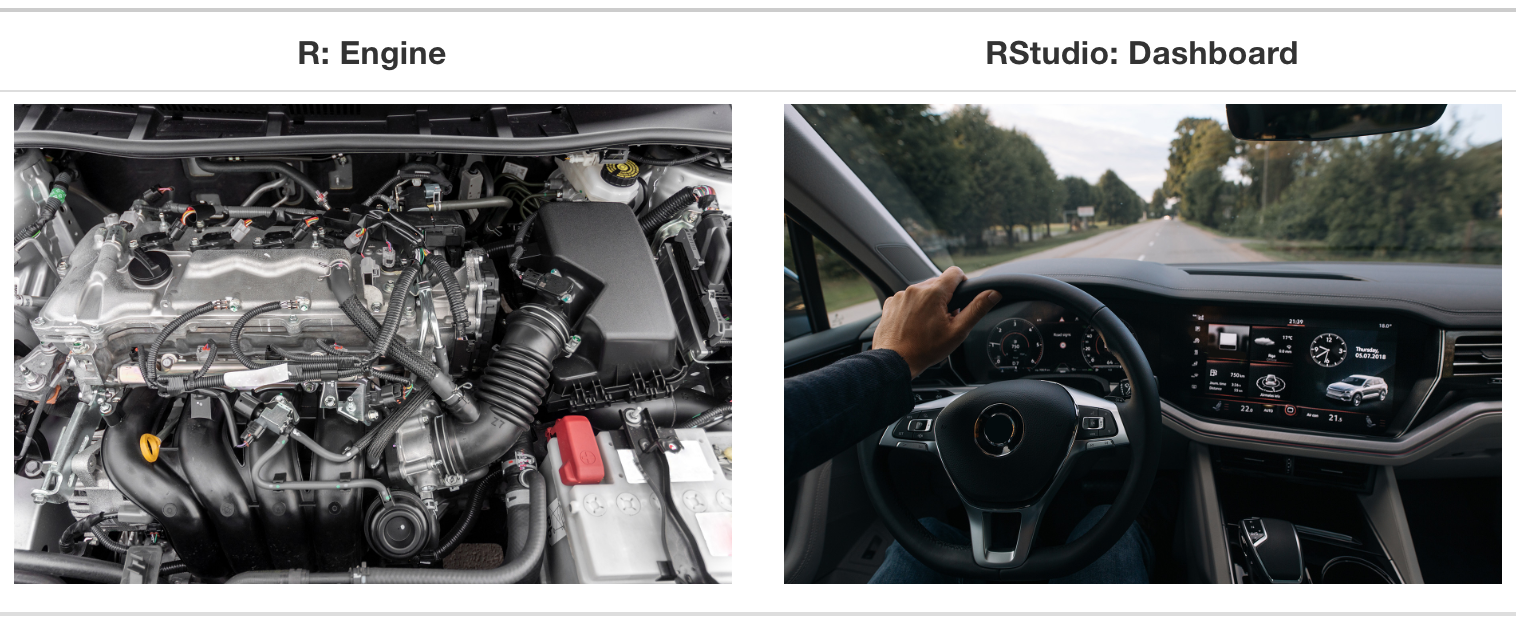
R is a free, open-source programming language specifically designed for statistical computing and graphics. It is widely used for data analysis, statistical modeling, and graphical representation of data.
RStudio, on the other hand, is an integrated development environment (IDE) for R. It enhances the user experience of R with a more accessible interface, featuring a viewable environment, file browser, data viewer, and plotting pane. RStudio simplifies the programming experience with integrated help, syntax highlighting, and context-aware tab completion.
First step: download and install R at https://cloud.r-project.org/.
Second step: Download and install Rstudio at https://posit.co/download/rstudio-desktop/
Third step: Open Rstudio instead of R
For beginners, familiarizing yourself with the interface can significantly streamline your learning and coding experience in R. Here is the breakdown of Rstudio’s main panels:
The Source Editor at the top-left: This is where you can write your R scripts. You can create, write, edit, and save R scripts here. To do so, click File on the top drop-down menus.
The Console Area at the bottom-left: The console area is where R code is executed interactively. You can either run a script from the Source Editor or type commands directly into the console, and the output or results are displayed in the Console. Note that if you type codes in the console, you will not be able to save them. This is why we use script files (which are save-able) instead of directly typing in the console.
The Environment and History Pane at the top-right:
Environment is your current workspace, including the datasets, variables, and other objects you have defined. It’s a great tool for keeping track of the data and functions you are working with.
History keeps a log of all the commands that have been run in the current session. You can browse through this history and re-run commands as needed.
The Miscellaneous Pane at the lower right.
Files: This tab allows you to navigate through the files in your working directory. You can open, delete, and organize your files from here.
Plots: When you create graphs and charts in R, they appear in this tab. You can also export these plots from here.
Packages: This tab shows the R packages you have installed and allows you to install new ones. R packages are collections of functions and datasets created by the R community. You will know how to install a package very soon.
Help: Provides access to R documentation and help files, which is invaluable for learning more about R functions and packages.If you need help on a particular command, you can type ? followed by the command in the console. For example, if you need help on the sum() command, type ?sum() in the console. R will pull out the documents regarding the sum() command, and it will show up at the Help tab at the lower right.
Viewer: Used to display local web content, like interactive R Markdown/Quarto outputs, shiny apps, and HTML widgets.
You might have already noticed that there are many helpful build-in settings in Rstudio. For example, you can import a dataset by clicking the Import Dataset button on the Environment panel instead of writing importing codes. You can also customize your script appearance. Just click the Tools on the settings banner, then Global Options and Appearance buttons.
To use a contributed package, you first need to install it.
After installation, a package is not immediately available in your R session. One more thing before we continue, we need to load the installed packages.
The following demonstrates how to install a prevalent data science R package, tidyverse, as an example. tidyverse is a collection of many other R packages used for many data analysis tasks. We will learn more about the tidyverse syntax in the next few weeks.
install.packages("tidyverse", repos="http://cran.us.r-project.org") package 'tidyverse' successfully unpacked and MD5 sums checked
The downloaded binary packages are in
C:\Users\zc3154\AppData\Local\Temp\RtmpUz7j0J\downloaded_packagesvignette("dplyr")The R community is active, and packages are regularly updated. You can update installed packages using functions like update.packages(). Of course, you can remove a package as well.
You can create your own packages. Of course, this requires some knowledge of R’s structure and conventions for package creation. This class is not about it.
It is important to stay organized of your scripts and other materials, like data and outputs, for an productive and reproducible workspace.
For example, by clicking the File drop-down menu, you can create a Project as a designated folder for your project.
Every time R runs, it has a working directory, which tells R where to load your files and data.
# Get the path of the current directory
getwd()
# Change the working directory
setwd("~/Rcourse") # ~/ indicates the user's home directory Depending on your operating system, you might need to use forward-slashes (/) rather than backslashes (\).
You are reading a Quarto file right now! Quarto is an innovative tool that combines your code and results and flows them in reproducible outputs with a variety of formats (e.g., PDFs, Word files, presentations, websites, and more).
It is a command line interface tool, not an R package. See Quarto.org to know more about it. You may use Quarto to create your own website!
Let’s start with two quick examples of what R can help with.
library(palmerpenguins) # we here use a dataset called "palmerpenguins", which is proviede as an R data package

#
data(package = 'palmerpenguins')
head(penguins)
# A tibble: 6 × 8
species island bill_length_mm bill_depth_mm flipper_length_mm body_mass_g
<fct> <fct> <dbl> <dbl> <int> <int>
1 Adelie Torgersen 39.1 18.7 181 3750
2 Adelie Torgersen 39.5 17.4 186 3800
3 Adelie Torgersen 40.3 18 195 3250
4 Adelie Torgersen NA NA NA NA
5 Adelie Torgersen 36.7 19.3 193 3450
6 Adelie Torgersen 39.3 20.6 190 3650
# ℹ 2 more variables: sex <fct>, year <int>
The following block of code computes the summary statistics by penguin species.
library(tidyverse)
penguins %>%
  group_by(species) %>%
  summarize(across(where(is.numeric), mean, na.rm = TRUE))
Warning: There was 1 warning in `summarize()`.
ℹ In argument: `across(where(is.numeric), mean, na.rm = TRUE)`.
ℹ In group 1: `species = Adelie`.
Caused by warning:
! The `...` argument of `across()` is deprecated as of dplyr 1.1.0.
Supply arguments directly to `.fns` through an anonymous function instead.
# Previously
across(a:b, mean, na.rm = TRUE)
# Now
across(a:b, \(x) mean(x, na.rm = TRUE))# A tibble: 3 × 6
species bill_length_mm bill_depth_mm flipper_length_mm body_mass_g year
<fct> <dbl> <dbl> <dbl> <dbl> <dbl>
1 Adelie 38.8 18.3 190. 3701. 2008.
2 Chinstrap 48.8 18.4 196. 3733. 2008.
3 Gentoo 47.5 15.0 217. 5076. 2008.We also use R for data visualizations. See the following visualization of exploring the relationship between the bill length and bill depth in a scatter plot.
library(ggplot2)


ggplot(data = penguins,
       aes(x = bill_length_mm, y = bill_depth_mm)) +
  geom_point(aes(color = species,
                 shape = species),
             size = 2)  +
  scale_color_manual(values = c("darkorange","darkorchid","cyan4"))
Warning: Removed 2 rows containing missing values or values outside the scale range
(`geom_point()`).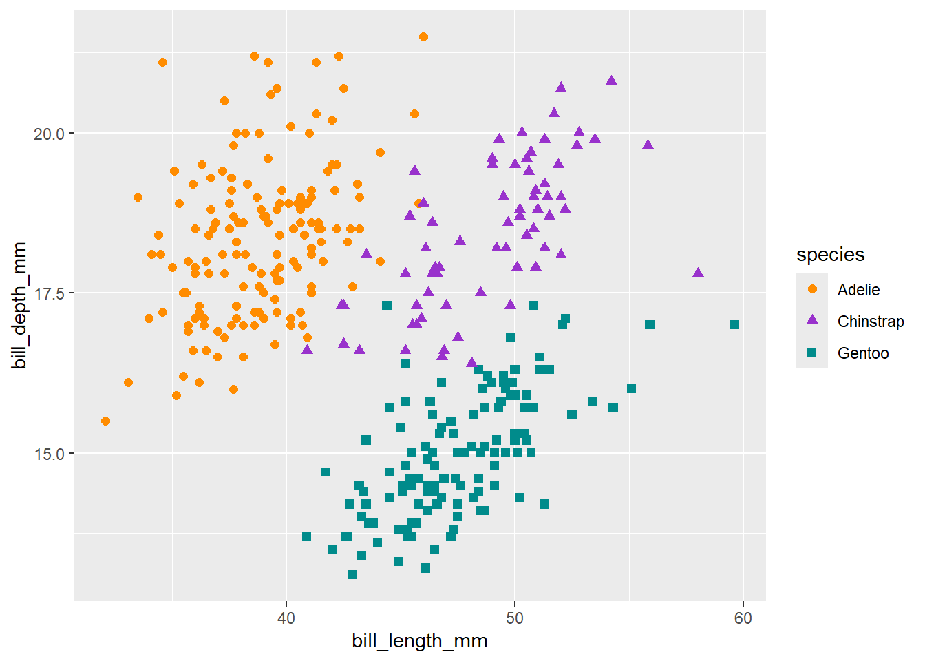
Further statistical test then can be performed in R to provide statistical inferences of the relationship between the bill length and bill depth.
cor.test(penguins$bill_length_mm, penguins$bill_depth_mm,
                    method = "pearson")
    Pearson's product-moment correlation

data:  penguins$bill_length_mm and penguins$bill_depth_mm
t = -4.4591, df = 340, p-value = 1.12e-05
alternative hypothesis: true correlation is not equal to 0
95 percent confidence interval:
 -0.3328072 -0.1323004
sample estimates:
       cor
-0.2350529 Warning: package 'visNetwork' was built under R version 4.3.3nb <- 25
nodes <- data.frame(id = 1:nb, label = paste("id", 1:nb),
group = sample(LETTERS[1:3], nb, replace = TRUE),
value = 1:nb,
title = paste("Edge", 1:nb), stringsAsFactors = FALSE)
edges <- data.frame(from = trunc(runif(nb)*(nb-1))+1,
to = trunc(runif(nb)*(nb-1))+1,
value = rnorm(nb, 10))visNetwork(nodes, edges, width="100%", height="400px", background="#eeefff",
main="Network", submain="And what a great network it is!",
footer= "Hyperlinks and mentions among media sources") |>
visEdges(arrows = 'from') |>
visLegend(useGroups = FALSE, addNodes = data.frame(label = "Nodes", shape = "circle"),
addEdges = data.frame(label = "link", color = "black")) |>
visOptions(highlightNearest = TRUE, nodesIdSelection = TRUE)Our goal is to write readable R codes to practice basic CSS applications. So, we may not use the strict terminologies that computer scientists or statisticians would use in writing complex codes and functions. We use a correct but colloquial language of R.
We start by building a basic data analysis workflow knowledge via the R tidyverse framework. We then head to text analysis and social network analysis. In this class, the content is mainly modified from the following resources. Check them out. These are great resources to start your journey of R for CSS!
Syntax simple rules:
Commands are separated by a new line or ;
Comment lines start with #
Case sensitive: d is not D
R can be used as a simple calculator. Let’s try some basic arithmetic operations.
# Addition.
3 + 2
[1] 53+0 [1] 3# Subtraction
5 - 2 [1] 3# Multiplication
4 *3[1] 12# Division
10 / 2[1] 5a <- 10 # the most commonly used assignment operator
b = 5
c <- a + b # Adding variables
d <<- 8 # an assignment operator that is used in functions. Don't worry about it now.
9 -> e
9 ->> fRe-assign value to an existing variable.
a<-11f=3
f==3 # equal to[1] TRUEWorking with GenAI
You can use GenAI to know and brainstorm the best practices of naming conventions in R.
Numeric variables can be integers, decimals, and fractions.
starting httpd help server ... doneCheck their data type.
Use either double or single quotation marks to represent string variables in R.
a<-"apple"
b<-"banana"
p<-"peach"e<-'This also works' #single quotation marks also work
e[1] "This also works"class(e)[1] "character"f<- "This does not work'" #Be consistent!
fIf there is a single quotation mark exists in the string variable, use double quotation. See examples below.
g <- "This also won't work'h<-"I'm happy that this works!"
h[1] "I'm happy that this works!"Another type is called logical, which are TRUE and FALSE. You may find it is also referred as “boolean” in other languages.
1+2>=3[1] TRUEc+d>=f[1] TRUEWhy k equals TRUE?
Data structure is about how you would store your data.
A vector is an ordered set of elements. You can create a vector of any data type, as long as all the elements in that vector have the same data type.
num.v<-1:6 # the most simple way to create a number sequence
str.v<-c("apple", "banana", "peach")
str.v<-c(a,b,p)


num.v
[1] 1 2 3 4 5 6str.v [1] "apple" "banana" "peach" How many elements in each of the vectors?
Working with GenAI
Try this in your console: “c(1, 2) + c(10, 20, 30, 40)”. What does this code do? Ask GenAI for help (i.e., annotate and explain).
Hint: “What is vector recycling in R? Provide an example.”
Factor is a data type or structure used to represent categorical variables, which can take on a limited number of distinct values (called levels). It can be used for creating a categorical variable, either nominal or ordinal.
hair_color <- c("Black", "Blonde", "Black", "Red", "Blonde")

hair_factor <- factor(hair_color)

hair_factor
[1] Black Blonde Black Red Blonde
Levels: Black Blonde RedThe default level orders are made alphabetically. You can also customize (i.e., specify) levels and further order them.
education <- factor(c("High School", "PhD", "Bachelor's"),
                   levels = c("High School", "Bachelor's", "Master's", "PhD"),
                   ordered = TRUE)

education
[1] High School PhD Bachelor's
Levels: High School < Bachelor's < Master's < PhDWorking with GenAI
Ask GenAI: “What is the difference between factors and character vectors in R? When should I use each? Please provide examples”
Matrices arrange numbers in rows and columns and are in rectangular shapes. We will be back for matrices for the text-as-data and social network analysis modules.
m[,1]
m <- matrix(data=2, nrow=4, ncol=3) # create a matrix of twos
m
[,1] [,2] [,3]
[1,] 2 2 2
[2,] 2 2 2
[3,] 2 2 2
[4,] 2 2 2m<-matrix(2,4,3)
m [,1] [,2] [,3]
[1,] 2 2 2
[2,] 2 2 2
[3,] 2 2 2
[4,] 2 2 2How about creating an identity matrix? An identity matrix is a matrix type that has all zeros except the diagonal elements that are ones.
     [,1] [,2] [,3] [,4] [,5]
[1,]    1    0    0    0    0
[2,]    0    1    0    0    0
[3,]    0    0    1    0    0
[4,]    0    0    0    1    0
[5,]    0    0    0    0    1
You can also assign elements. Notice that the matrix is filled by column orders by default. But you can specify the order.
p<-matrix(num.v, 2, 3)
p
[,1] [,2] [,3]
[1,] 1 3 5
[2,] 2 4 6q<-matrix(num.v, 2, 3, byrow=TRUE)
q [,1] [,2] [,3]
[1,] 1 2 3
[2,] 4 5 6You can convert a matrix to a vector. Notice the order of elements.
Of course, you can have matrices that has elements other than numeric.
char_m <- matrix(letters[1:6], 2, 3)
char_m
[,1] [,2] [,3]
[1,] "a" "c" "e"
[2,] "b" "d" "f" Combine vectors or matrices into a matrix
r<-rbind(p,q) #bind two matrices by rows; append
r
[,1] [,2] [,3]
[1,] 1 3 5
[2,] 2 4 6
[3,] 1 2 3
[4,] 4 5 6s<-cbind(p,q) #bind two matrices by columns; merge
s [,1] [,2] [,3] [,4] [,5] [,6]
[1,] 1 3 5 1 2 3
[2,] 2 4 6 4 5 6A List is an ordered set of components. It might sound similar to a vector. However, you can include any types of data in a list.
l<-list(k, num.v, str.v, id_m)
l
[[1]]
[1] TRUE
[[2]]
[1] 1 2 3 4 5 6
[[3]]
[1] "apple" "banana" "peach"
[[4]]
[,1] [,2] [,3] [,4] [,5]
[1,] 1 0 0 0 0
[2,] 0 1 0 0 0
[3,] 0 0 1 0 0
[4,] 0 0 0 1 0
[5,] 0 0 0 0 1Date frames are used to store tabular data, which is made up of three principal components, the columns, the rows, and the data.
Following are the basic characteristics of a data frame:
The column names (i.e., variable names) should be non-empty.
The row names (e.g., identify numbers) should be unique.
The data stored in a data frame can be of numeric, factor or character type.
Each column should contain same number of data items.
# Creating a fake dataset
families <- data.frame(
  family_id = 1:10,
  num_children = c(2, 3, 1, 4, 2, 3, 1, 2, 0, 3),
  annual_income = c(45000, 52000, 48000, 55000, 43000, 50000, 47000, 51000, 53000, 44000),
  health_score = c(80, 85, 78, 90, 75, 88, 82, 79, 91, 77)
)View(families)
families family_id num_children annual_income health_score
1 1 2 45000 80
2 2 3 52000 85
3 3 1 48000 78
4 4 4 55000 90
5 5 2 43000 75
6 6 3 50000 88
7 7 1 47000 82
8 8 2 51000 79
9 9 0 53000 91
10 10 3 44000 77Let’s explore the structure of this data frame.
str(families) 'data.frame': 10 obs. of 4 variables:
$ family_id : int 1 2 3 4 5 6 7 8 9 10
$ num_children : num 2 3 1 4 2 3 1 2 0 3
$ annual_income: num 45000 52000 48000 55000 43000 50000 47000 51000 53000 44000
$ health_score : num 80 85 78 90 75 88 82 79 91 77The first and last six rows of this data.
head(families,n=3) family_id num_children annual_income health_score
1 1 2 45000 80
2 2 3 52000 85
3 3 1 48000 78tail(families,n=8) family_id num_children annual_income health_score
3 3 1 48000 78
4 4 4 55000 90
5 5 2 43000 75
6 6 3 50000 88
7 7 1 47000 82
8 8 2 51000 79
9 9 0 53000 91
10 10 3 44000 77nrow(families)[1] 10Descriptive statistics summarize and describe the features of a data set.
It’s the sum of all data points divided by the number of points.
mean(families$annual_income)[1] 48800Working with GenAI
GenAI can help explain function arguments. See example below:
values<-c(1,2,NA,4)
mean(values, na.rm=TRUE)
You may ask GenAI: ““What does the na.rm argument do in the mean() function?”
The middle value in a sorted list is called median.
median(families$annual_income)[1] 49000Measures the amount of variation in a set of values.
sd(families$annual_income)[1] 4049.691The square of the standard deviation.
var(families$annual_income)[1] 16400000summary(families) family_id num_children annual_income health_score
Min. : 1.00 Min. :0.00 Min. :43000 Min. :75.00
1st Qu.: 3.25 1st Qu.:1.25 1st Qu.:45500 1st Qu.:78.25
Median : 5.50 Median :2.00 Median :49000 Median :81.00
Mean : 5.50 Mean :2.10 Mean :48800 Mean :82.50
3rd Qu.: 7.75 3rd Qu.:3.00 3rd Qu.:51750 3rd Qu.:87.25
Max. :10.00 Max. :4.00 Max. :55000 Max. :91.00 As we wrap up our first session, I hope you had a chance to know the R environment and RStudio settings, along with an understanding of writing base R codes. These foundation elements will serve as the building blocks for your journey in data analysis with R.
Our next R session will start with an overview of a typical data analysis workflow of using tidyverse. Looking forward to seeing you all in our next R session!